Byte Pair Encoding (BPE) Algorithm: A Deep Technical Analysis for Modern NLP

Byte Pair Encoding, BPE algorithm, subword tokenization, NLP tokenization, GPT tokenization, BERT tokenizer

---

Table of Contents

1. Executive Summary
2. The Vocabulary Problem in NLP
3. Algorithmic Foundations of BPE
4. Step-by-Step BPE Training Process
5. Tokenization Inference: Encoding New Text
6. Implementation Deep Dive
7. Advanced Variants and Optimizations
8. BPE in Modern LLM Architectures
9. Performance Analysis and Complexity
10. Common Pitfalls and Edge Cases
11. Conclusion and Future Directions

---

Executive Summary

Byte Pair Encoding (BPE) represents a paradigm shift in how neural networks process human language. Originally developed as a data compression technique by Philip Gage in 1994, BPE was adapted for Natural Language Processing by Sennrich et al. in 2016, fundamentally solving the open vocabulary problem that plagued statistical machine translation systems.

Unlike character-level tokenization (which loses semantic meaning) and word-level tokenization (which cannot handle out-of-vocabulary words), BPE operates on a subword level, learning an optimal vocabulary through data-driven merge operations. This approach achieves an elegant balance: rare words are decomposed into meaningful units, while common words remain intact as single tokens.

Technical Significance:

• Vocabulary Size Control: Fixed-size vocabulary (typically 32K-100K tokens) regardless of corpus size
• OOV Robustness: Zero out-of-vocabulary rate for any text
• Morphological Awareness: Automatically learns prefixes, suffixes, and root words
• Cross-lingual Efficiency: Shared vocabulary spaces across multiple languages

---

The Vocabulary Problem in NLP

The Open Vocabulary Challenge

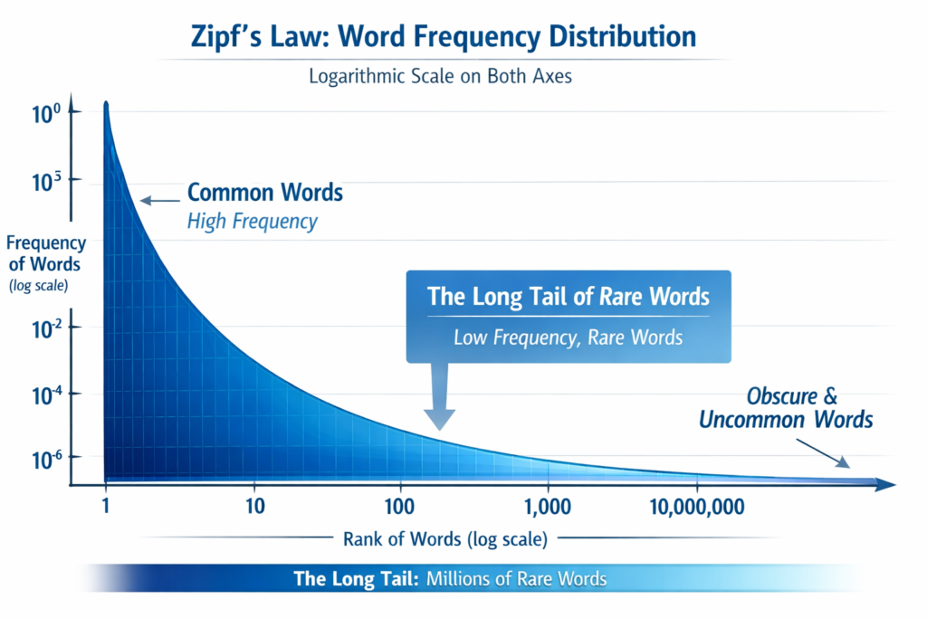
Natural language exhibits Zipf’s Law: a small number of words appear frequently, while the vast majority appear rarely. In large corpora:

• The top 100 English words cover ~50% of all tokens
• Words appearing ≤10 times constitute >60% of unique vocabulary entries
• Proper nouns, technical terms, and morphological variations create infinite vocabulary expansion

Limitations of Traditional Approaches

Table

Copy

Approach	Drawbacks	Example Failure Case
Word-level	Infinite vocabulary, massive embedding matrices	“ChatGPT-4.5-turbo” → OOV
Character-level	Loss of semantic meaning, longer sequences	“unhappiness” → 11 tokens
Morpheme-based	Requires linguistic expertise, language-specific	Cannot handle neologisms

BPE solves this by treating the vocabulary as a learned compression codebook, where frequent character sequences are merged into single symbols through an iterative optimization process.

---

Algorithmic Foundations of BPE

Core Mathematical Formulation

BPE defines an optimization problem over a corpus C and target vocabulary size V :

Objective: Find vocabulary V and segmentation S that minimize: L=∑w∈C​∣S(w)∣+λ∣V∣

Where:

• ∣S(w)∣ = number of tokens for word w
• ∣V∣ = vocabulary size
• λ = regularization hyperparameter (implicitly controlled by V )

The Greedy Approximation

Since finding the global optimum is NP-hard (related to the shortest common supersequence problem), BPE employs a greedy frequency-based heuristic:

1. Initialization: Start with character vocabulary V0​={c∣c∈Σ}
2. Iteration: For i=1 to V−∣Σ∣ :
   • Find most frequent adjacent pair (x,y) in current tokenization
   • Create new symbol z=xy
   • Update Vi​=Vi−1​∪{z}
   • Replace all occurrences of (x,y) with z

This is essentially Huffman coding on character bigrams, but with a critical difference: BPE merges are applied deterministically and globally across the corpus, creating a context-free grammar for tokenization.

Information-Theoretic Interpretation

Each merge operation reduces the entropy of the token sequence:

H(Ti​)=H(Ti−1​)−I(X;Y)

Where I(X;Y) is the mutual information between adjacent symbols X and Y . BPE greedily maximizes information gain at each step, though this doesn’t guarantee global entropy minimization.

---

Step-by-Step BPE Training Process

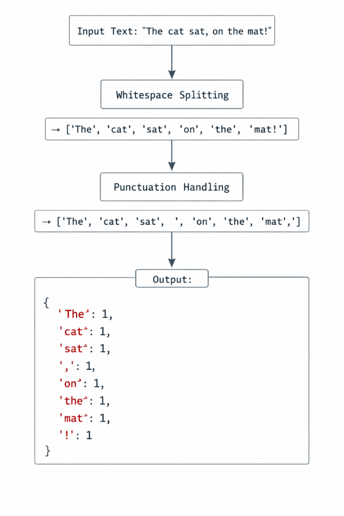
Phase 1: Preprocessing and Word Frequency Extraction

Before BPE training, the corpus undergoes pre-tokenization (typically whitespace and punctuation splitting):

Python

# Simplified pre-tokenization
corpus = {
    "low": 5, "lower": 2, "lowest": 1,
    "new": 6, "newer": 3, "newest": 2,
    "wide": 3, "wider": 2, "widest": 1
}

End-of-Word Marker: A special symbol </w> (or Ġ in GPT-2) is appended to mark word boundaries. This prevents cross-word merging and distinguishes word-final subwords from internal ones.

Phase 2: Character-Level Initialization

Convert each word into a character sequence:

"low</w>" → l o w </w>
"lower</w>" → l o w e r </w>
"lowest</w>" → l o w e s t </w>

Initial vocabulary: {l,o,w,e,r,s,t,</w>}

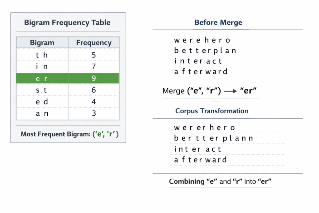
Phase 3: Iterative Merge Operations

Iteration 1:

• Count all adjacent pairs across corpus
• ('l', 'o'): 10 occurrences (5+2+1+6+3+2 = wait, let’s calculate properly)

Actually, let’s trace correctly:

• “low” (5): l-o, o-w, w-
• “lower” (2): l-o, o-w, w-e, e-r, r-
• “lowest” (1): l-o, o-w, w-e, e-s, s-t, t-
• “new” (6): n-e, e-w, w-
• “newer” (3): n-e, e-w, w-e, e-r, r-
• “newest” (2): n-e, e-w, w-e, e-s, s-t, t-
• “wide” (3): w-i, i-d, d-e, e-
• “wider” (2): w-i, i-d, d-e, e-r, r-
• “widest” (1): w-i, i-d, d-e, e-s, s-t, t-

Most frequent pair: ('e', 'r') with 5 occurrences (lower×2, newer×3)

Create merge rule: ('e', 'r') → 'er'

Update corpus:

• “lower” → l o w er
• “newer” → n e w er
• “wider” → w i d er

Iteration 2: Now count pairs again with updated tokenization…

• ('l', 'o'): 5+2+1 = 8
• ('o', 'w'): 5+2+1 = 8
• ('w', '</w>'): 5+6 = 11 ← New most frequent

Merge: ('w', '</w>') → 'w</w>'

This creates a word-final “w” token, distinguishing it from internal “w”.

Iteration 3-10: Continue until vocabulary size reaches target (e.g., 10,000 merges).

Phase 4: Vocabulary and Merge Table Serialization

The final output consists of:

1. Vocabulary File: List of all tokens (base characters + merged symbols)
2. Merge Table: Ordered list of merge operations (critical for deterministic encoding)

JSON

{
  "vocab": {
    "l": 0, "o": 1, "w": 2, "e": 3, "r": 4, 
    "s": 5, "t": 6, "</w>": 7, "er": 8, 
    "w</w>": 9, "ow": 10, "lo": 11, ...
  },
  "merges": [
    ["e", "r"], ["w", "</w>"], ["o", "w"], 
    ["l", "o"], ["n", "e"], ...
  ]
}

Critical Insight: The merge order matters! If we merged ('o', 'w') before ('l', 'o'), we’d get different tokens. BPE’s determinism relies on strict frequency-based ordering.

---

Tokenization Inference: Encoding New Text

Training creates the vocabulary; inference applies it to new text. This is where BPE’s greedy longest-match strategy operates.

The Encoding Algorithm

Given input text T and merge table M=[m1​,m2​,…,mk​] :

Python

def encode(text, merges):
    # 1. Pre-tokenize
    words = pre_tokenize(text)
    
    tokens = []
    for word in words:
        # 2. Initialize as characters + end marker
        word_tokens = list(word) + ['</w>']
        
        # 3. Apply merges in order of priority
        for merge_pair in merges:
            i = 0
            while i < len(word_tokens) - 1:
                if (word_tokens[i], word_tokens[i+1]) == merge_pair:
                    # Apply merge
                    word_tokens = (word_tokens[:i] + 
                                  [merge_pair[0] + merge_pair[1]] + 
                                  word_tokens[i+2:])
                else:
                    i += 1
        
        tokens.extend(word_tokens)
    
    return tokens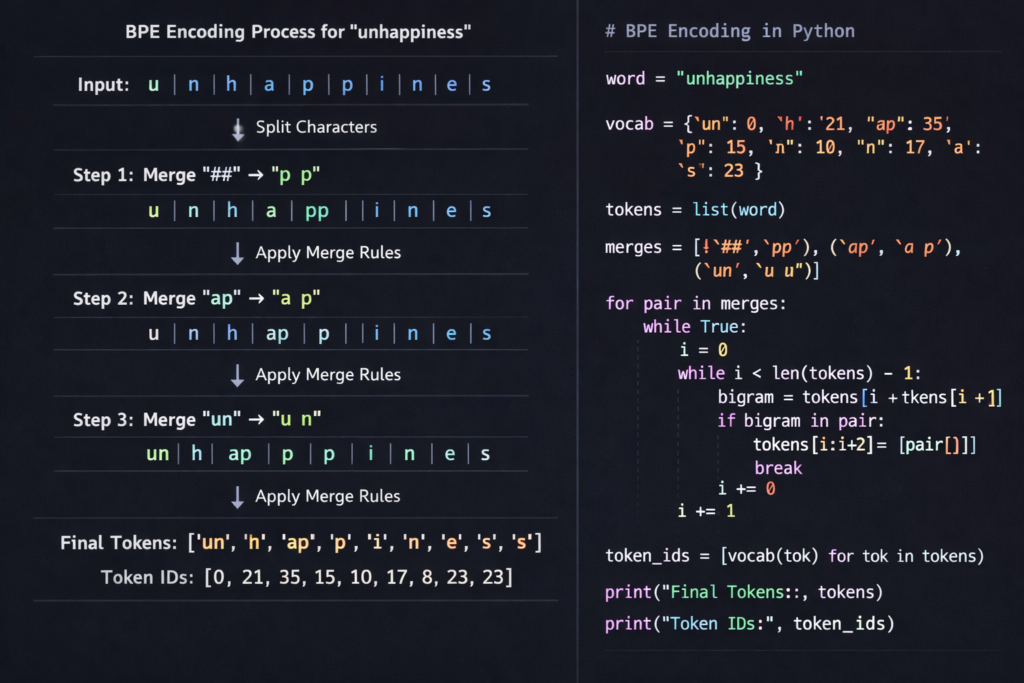

Determinism and Ambiguity Resolution

Consider the word “thinner”:

• Characters: t-h-i-n-n-e-r-
• Possible merges: ('n', 'n') vs ('i', 'n')

BPE resolves this through merge priority (frequency). If ('n', 'n') was merged earlier in training (higher frequency), it takes precedence:

Step 1: t h i n n e r </w>
Step 2: t h i nn e r </w>  # ('n','n') merged first
Step 3: t h i nn er </w>   # ('e','r') next
...

This deterministic approach ensures identical tokenization across different implementations.

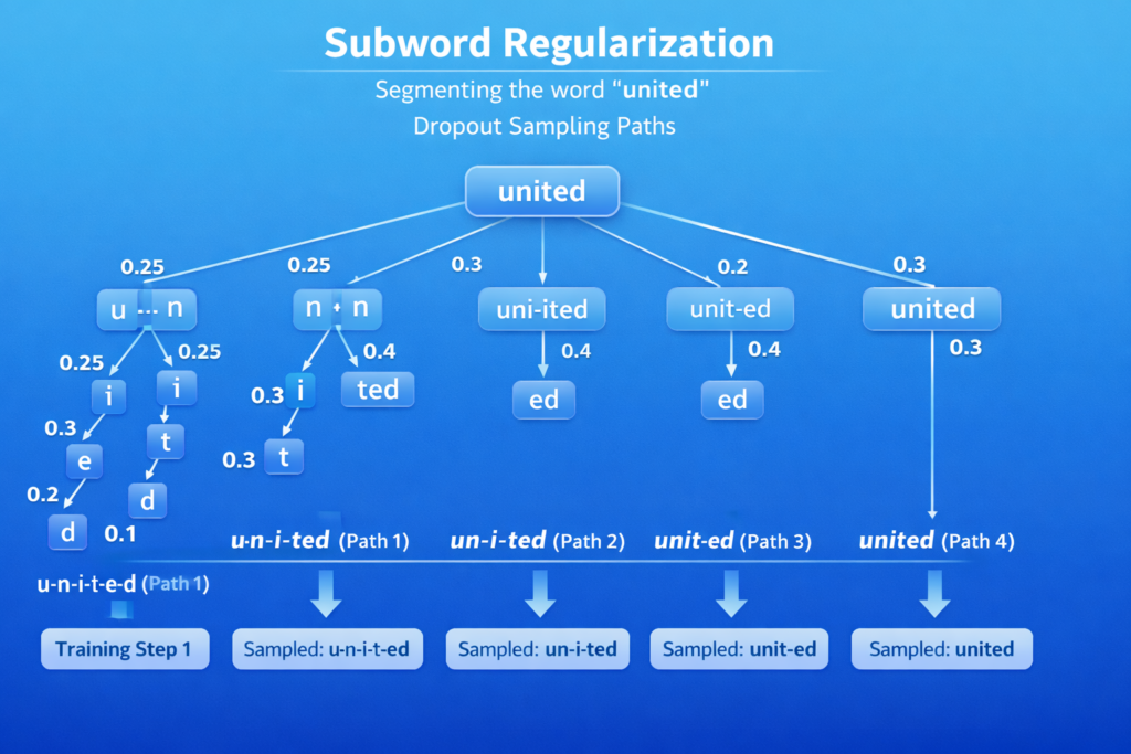
Subword Regularization: The Dropout Variation

Standard BPE is deterministic, but subword regularization (Kudo, 2018) introduces stochasticity during training:

P(S∣X)=∏(x,y)∈S​count(x)⋅count(y)count(xy)​

Where S is a segmentation path. During training, sample segmentations proportional to their probability, improving robustness for languages with ambiguous segmentation (Japanese, Chinese).

---

Implementation Deep Dive

Memory-Efficient Training with Priority Queues

Naive BPE implementation has O(N2⋅V) complexity. Optimized implementations use:

1. Pair Counting with Hash Maps: O(1) frequency updates
2. Max-Heap for Merge Selection: O(logV) extraction of highest-frequency pair
3. Lazy Evaluation: Only recompute frequencies for affected positions

Python

import heapq
from collections import defaultdict

class BPETrainer:
    def __init__(self, vocab_size):
        self.vocab_size = vocab_size
        self.merge_rules = []
        
    def train(self, corpus):
        # Build initial pair frequencies
        pair_counts = defaultdict(int)
        word_tokens = {}  # word -> list of tokens
        
        for word, freq in corpus.items():
            tokens = list(word) + ['</w>']
            word_tokens[word] = tokens
            
            for i in range(len(tokens) - 1):
                pair = (tokens[i], tokens[i+1])
                pair_counts[pair] += freq
        
        # Max-heap (using negative for Python's min-heap)
        heap = [(-count, pair) for pair, count in pair_counts.items()]
        heapq.heapify(heap)
        
        while len(self.merge_rules) < self.vocab_size:
            # Get highest frequency pair
            neg_count, best_pair = heapq.heappop(heap)
            
            # Verify count is current (lazy deletion)
            current_count = self._get_pair_count(best_pair, word_tokens, corpus)
            if -neg_count != current_count:
                heapq.heappush(heap, (-current_count, best_pair))
                continue
            
            # Apply merge
            self._apply_merge(best_pair, word_tokens)
            self.merge_rules.append(best_pair)
            
            # Update affected pairs
            self._update_heap(best_pair, word_tokens, heap, corpus)
    
    def _apply_merge(self, pair, word_tokens):
        new_symbol = pair[0] + pair[1]
        for word, tokens in word_tokens.items():
            i = 0
            new_tokens = []
            while i < len(tokens):
                if i < len(tokens) - 1 and (tokens[i], tokens[i+1]) == pair:
                    new_tokens.append(new_symbol)
                    i += 2
                else:
                    new_tokens.append(tokens[i])
                    i += 1
            word_tokens[word] = new_tokens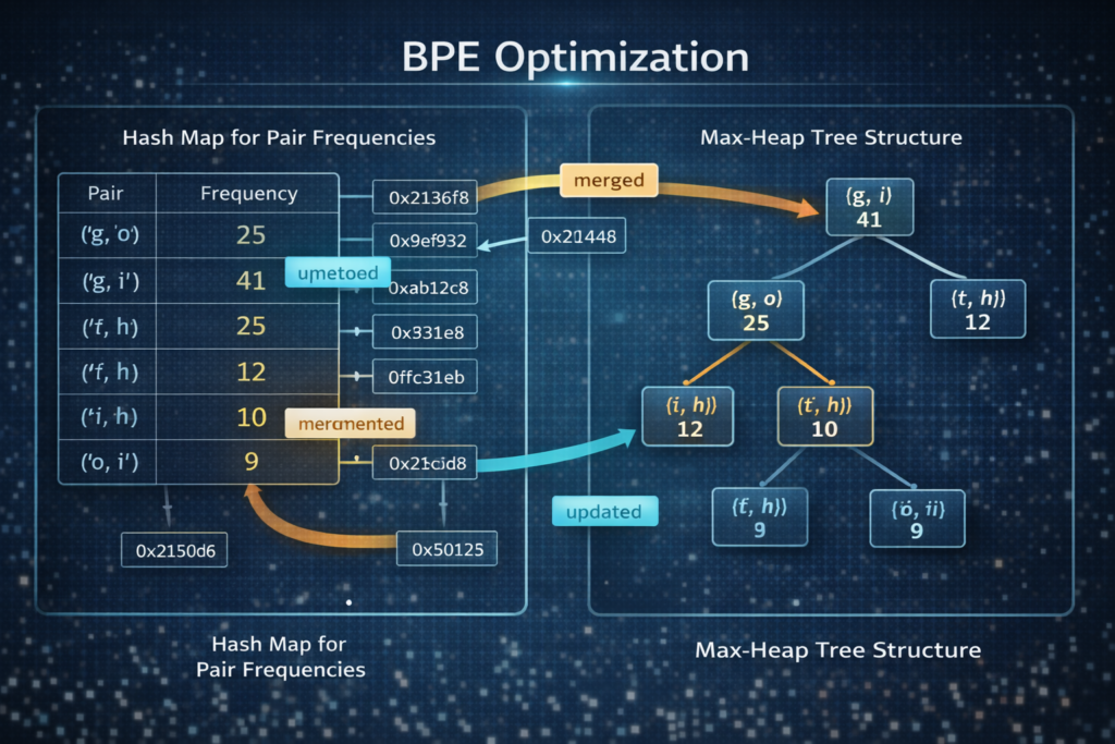

Byte-Level BPE (BBPE)

GPT-2 and RoBERTa use Byte-Level BPE, which operates on UTF-8 bytes rather than Unicode characters:

Advantages:

• Universal Coverage: Handles any Unicode character without OOV
• Vocabulary Size: Base vocabulary of 256 bytes + merges
• Consistency: No character normalization issues

Implementation:

Python

def bytes_to_unicode():
    """
    Returns mapping from UTF-8 bytes to Unicode strings.
    Avoids control characters and whitespace for readability.
    """
    bs = list(range(ord("!"), ord("~")+1)) + \
         list(range(ord("¡"), ord("¬")+1)) + \
         list(range(range(ord("®"), ord("ÿ")+1))
    cs = bs[:]
    n = 0
    for b in range(2**8):
        if b not in bs:
            bs.append(b)
            cs.append(2**8 + n)
            n += 1
    return dict(zip(bs, map(chr, cs)))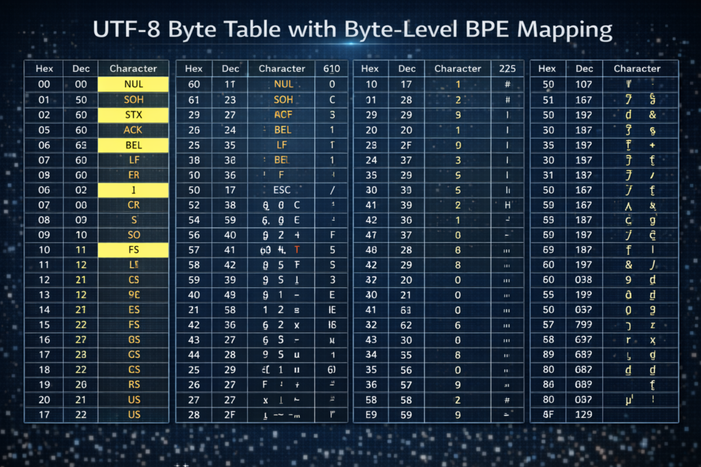

---

Advanced Variants and Optimizations

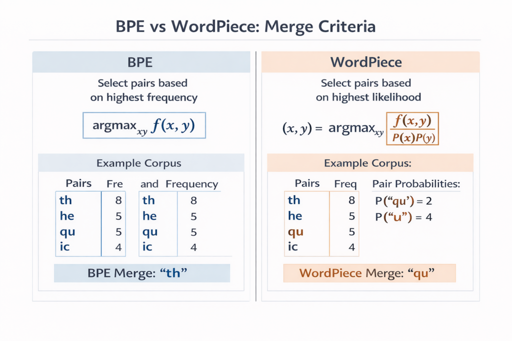
WordPiece: BPE’s Probability-Based Cousin

Used in BERT and DistilBERT, WordPiece modifies the merge criterion:

BPE Criterion:argmax(x,y)​count(x,y)

WordPiece Criterion:argmax(x,y)​count(x)⋅count(y)count(xy)​

This maximizes the likelihood of the training data rather than frequency, theoretically producing better segmentations for language modeling.

Unigram Language Model Tokenization

SentencePiece’s Unigram model approaches the problem differently:

1. Start with massive seed vocabulary (all substrings)
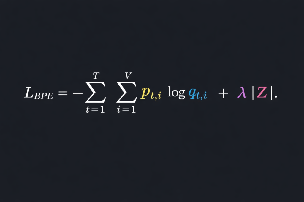
2. Iteratively remove tokens to minimize loss: L=−∑s∈S​logP(s)+λ∣V∣

Where P(s) is the unigram probability of subword s .

Advantages over BPE:

• Multiple segmentation candidates (via Viterbi algorithm)
• Better handling of morphologically rich languages
• Language-agnostic (no pre-tokenization required)

BPE Dropout and Robustness

Proposed by Provilkov et al. (2020), BPE Dropout randomly skips merge operations during training with probability p :

Python

def encode_with_dropout(word, merges, dropout_prob=0.1):
    tokens = list(word) + ['</w>']
    for merge in merges:
        if random.random() < dropout_prob:
            continue  # Skip this merge
        # Apply merge normally...

This creates multiple valid segmentations for the same word, improving model robustness and handling of rare words.

---

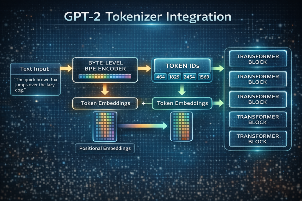
BPE in Modern LLM Architectures

GPT-2/GPT-3 Tokenizer Analysis

OpenAI’s GPT-2 uses a 50,257-token vocabulary:

• 50,000 merge operations
• 256 byte tokens
• 1 special token (<|endoftext|>)

Key Design Decisions:

• No <UNK> token (purely subword)
• Whitespace collapsed to Ġ (byte 288)
• Numbers split digit-by-digit (prevents massive vocabulary for numbers)

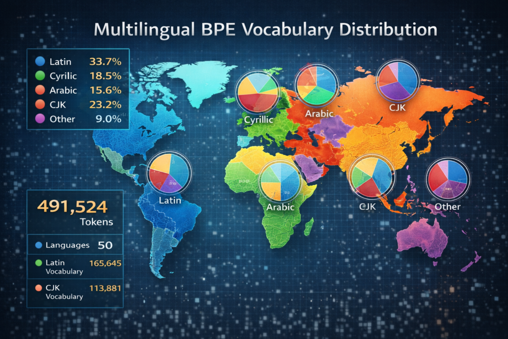
Multilingual BPE: mBERT and XLM-R

Cross-lingual models face the script imbalance problem:Table

Language	Script	Unique Characters	Training Data
English	Latin	26	300B tokens
Chinese	Han	50,000+	30B tokens
Arabic	Arabic	28	20B tokens

Solution: Script-aware sampling and vocabulary allocation:

• mBERT: Shared vocabulary with proportional allocation
• XLM-R: SentencePiece with alpha smoothing (α=0.3 ) to upsample low-resource languages

Tokenization Artifacts and Mitigation

The “SolidGoldMagikarp” Problem: Some BPE tokens become “glitched” during training—sequences that never appear in training data but exist in vocabulary. In GPT-2, the token ” SolidGoldMagikarp” (a Reddit username) triggered anomalous behavior because it was in the vocabulary but the model never learned meaningful representations.

Mitigation Strategies:

• Frequency Filtering: Only include tokens appearing ≥k times
• Hash-based Bucketing: Rare words → hash buckets (Google’s approach)
• Dynamic Vocabulary: Retrain tokenizers on specific domains

---

Performance Analysis and Complexity

Computational Complexity

Phase	Time Complexity	Space Complexity
Training	O(N⋅V⋅logV)	O(N⋅L)
Inference	O(L⋅V)	O(L)

Where:

• N = corpus size (token count)
• V = vocabulary size
• L = average word length

Optimization: For inference, use trie-based or Aho-Corasick string matching to achieve O(L) time regardless of vocabulary size.

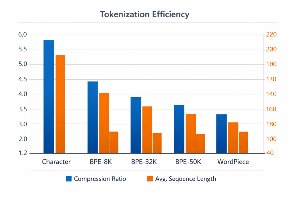
Compression Efficiency

BPE achieves compression ratios of 4:1 to 10:1 compared to character-level:Table

Tokenization	Avg Token Length	Sequence Length (1000 chars)
Character	1 byte	1000
BPE (32K vocab)	4.5 bytes	~220
BPE (50K vocab)	5.2 bytes	~190

Cache Optimization

Modern implementations use LRU caches for tokenization:

from functools import lru_cache

@lru_cache(maxsize=100000)
def tokenize_word(word):
    # BPE encoding logic
    return tuple(tokens)

Hit rates of 80-90% are typical for natural language due to repetition of common words.

---

Common Pitfalls and Edge Cases

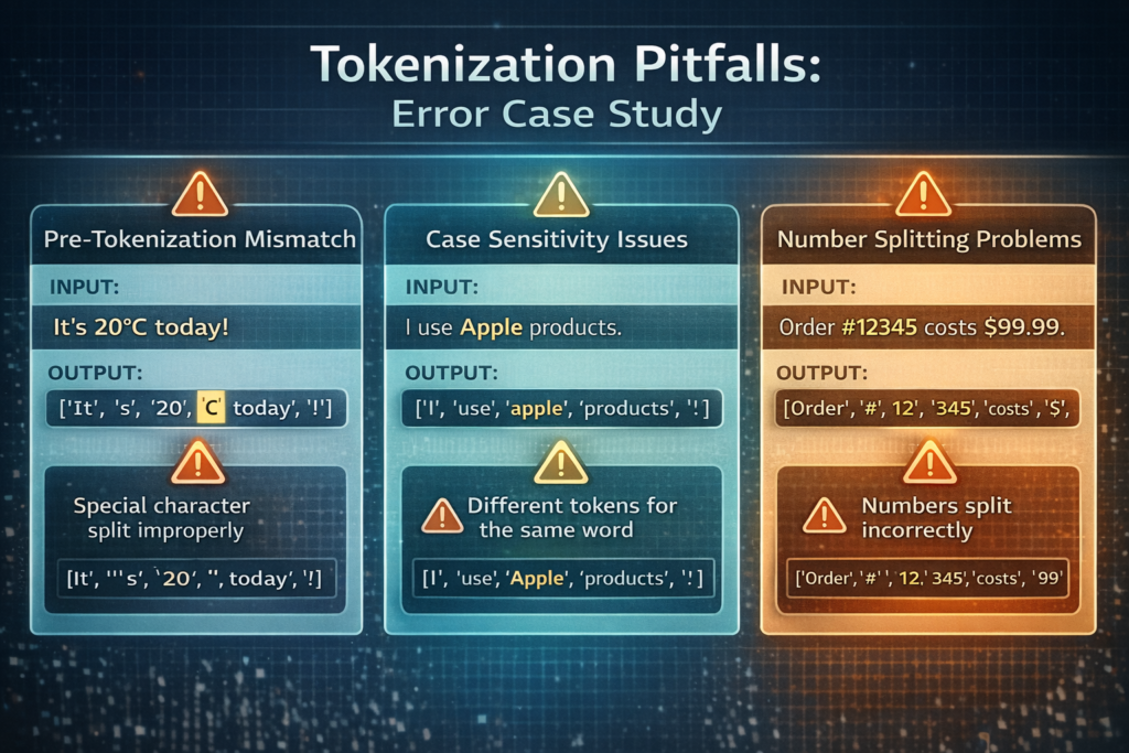
1. The Pre-tokenization Trap

BPE requires consistent pre-tokenization between training and inference. Mismatches cause silent errors:

Python

# Training: splits on whitespace only
train_tokens = text.split(' ')

# Inference: splits on punctuation
infer_tokens = re.findall(r'\w+|[^\w\s]', text)  # DISASTER!

Solution: Serialize pre-tokenization rules with the model.

2. Case Sensitivity

GPT-2 treats “The” and “the” differently:

• “The” → [“The”]
• “the” → [“Ġthe”] (with leading space marker)

This doubles vocabulary usage for cased languages. Lowercasing before BPE is common but loses information (proper nouns, emphasis).

3. Number Tokenization

Standard BPE splits numbers digit-by-digit:

• “2024” → [“2”, “0”, “2”, “4”] (GPT-2)
• “2024” → [“2024”] (if seen frequently in training)

This hurts arithmetic capabilities. Number-aware BPE (NBBPE) treats digit sequences as atomic units.

4. Adversarial Examples

Small character changes can drastically alter tokenization:

Python

Copy

"OpenAI" → ["Open", "AI"]  # 2 tokens
"OpenAİ" → ["Open", "A", "İ"]  # 3 tokens (Turkish dotted I)

This enables tokenization attacks on NLP systems by using visually similar Unicode characters.

---

Conclusion and Future Directions

Byte Pair Encoding represents a foundational algorithm in modern NLP, bridging the gap between character and word-level representations. Its elegance lies in the simplicity of the greedy merge heuristic combined with sophisticated implementation optimizations.

Key Takeaways:

1. Data-Driven: BPE learns vocabulary from corpus statistics, not linguistic rules
2. Deterministic: Identical training produces identical tokenization
3. Extensible: Variants like WordPiece and Unigram address specific limitations
4. Universal: Byte-level variants handle any language or symbol

Emerging Research:

• Differentiable Tokenization: Learning tokenization end-to-end with the model (STokenizer, 2023)
• Neural BPE: Using small networks to predict merge decisions
• Adaptive Vocabularies: Dynamic vocabulary adjustment during training

As we move toward multimodal LLMs processing text, images, and audio, BPE’s principles extend to visual tokenization (VQ-VAE codebooks) and audio tokenization (SoundStream). The subword philosophy—balancing granularity and semantics—remains the gold standard for discrete representation learning.

---

References and Further Reading

1. Sennrich, R., Haddow, B., & Birch, A. (2016). Neural Machine Translation of Rare Words with Subword Units. ACL.
2. Radford, A., et al. (2019). Language Models are Unsupervised Multitask Learners. OpenAI Technical Report.
3. Kudo, T. (2018). Subword Regularization: Improving Neural Network Translation Models with Multiple Subword Candidates. ACL.
4. Provilkov, I., et al. (2020). BPE-Dropout: Simple and Effective Subword Regularization. ACL.
5. Gage, P. (1994). A New Algorithm for Data Compression. C Users Journal.