How ChatGPT Works: Deep Technical Architecture of LLMs (2024)

An in-depth technical exploration of transformer architectures, tokenization, attention mechanisms, and the inference pipeline that powers modern conversational AI

---

Table of Contents

1. Introduction: The Illusion of Intelligence
2. The Transformer Revolution: Foundational Architecture
3. Tokenization: The First Critical Step
4. The Forward Pass: From Input to Output
5. Attention Mechanisms: The Core Innovation
6. Layer-by-Layer Processing
7. The Inference Pipeline: Step-by-Step
8. Decoding Strategies: From Probabilities to Text
9. Training vs. Inference: Key Differences
10. Hardware and Optimization
11. Conclusion and Future Directions

---

Introduction: The Illusion of Intelligence

When you type “Explain quantum computing” into ChatGPT and receive a coherent, contextually relevant response within milliseconds, you’re witnessing one of the most sophisticated computational processes ever engineered. What appears as “understanding” is actually a complex orchestration of matrix multiplications, probabilistic sampling, and hierarchical pattern recognition across billions of parameters.

This article provides a comprehensive technical deep-dive into the complete pipeline—from the moment your keystrokes are registered to the final token generation. We’ll examine the actual mathematical operations, memory structures, and computational graphs that enable modern Large Language Models (LLMs) to function.

The Deep Technical Architecture of Large Language Models: A Complete Guide to How ChatGPT and Modern AI Systems Work

---

The Transformer Revolution: Foundational Architecture

The Encoder-Decoder Paradigm

Modern LLMs like GPT-4, Claude, and Llama are built upon the transformer architecture introduced in Vaswani et al.’s seminal 2017 paper, “Attention Is All You Need.” While the original paper proposed an encoder-decoder structure for machine translation, autoregressive decoder-only models (GPT family) have become dominant for generative tasks.

Core Architectural Components:

1. Token Embeddings: Convert discrete tokens to continuous vector representations
2. Positional Encodings: Inject sequence order information
3. Transformer Blocks: Stacked layers of self-attention and feed-forward networks
4. Layer Normalization: Stabilize training and inference dynamics
5. Output Projection: Map final hidden states to vocabulary logits

Model Specifications (Approximate)

Model	Parameters	Layers	Hidden Size	Attention Heads	Context Window
GPT-3	175B	96	12,288	96	2,048
GPT-4 (estimated)	~1.8T (MoE)	120	~10,000	~128	128,000
Llama 3 70B	70B	80	8,192	64	128,000
Claude 3 Opus	~175B	~80	~12,000	~100	200,000

---

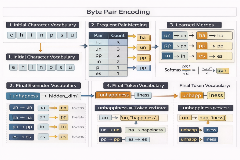
Tokenization: The First Critical Step

Before any neural processing occurs, your text input undergoes tokenization—a deterministic subword segmentation algorithm. This is not merely “splitting by spaces” but a sophisticated compression scheme learned from training data.

Byte Pair Encoding (BPE) Algorithm

Deep Dive in this topic – Byte Pair Encoding

Modern LLMs use Byte Pair Encoding or its variants (WordPiece, SentencePiece, TikToken):

1. Initialization: Start with character vocabulary (typically 256 byte values)
2. Merging: Iteratively merge most frequent adjacent pairs
3. Vocabulary Growth: Continue until target vocabulary size (typically 32,000-200,000 tokens)
4. Encoding: Greedy longest-match segmentation during inference

Technical Example:

Input: "Tokenization is fundamental"

Tokenization process:

• “Token” → [token_id: 15496]
• “ization” → [token_id: 318]
• ” is” → [token_id: 318] (note leading space)
• ” fundamental” → [token_id: 4060]

Result: [15496, 318, 318, 4060] (4 tokens)

Critical Implementation Details:

• Pre-tokenization: Regex patterns split on whitespace and punctuation
• Special Tokens: <|endoftext|>, <|im_start|>, <|im_end|> for conversation formatting
• Byte Fallback: Unknown characters encoded as byte sequences
• Efficiency: Average 0.75 words per token for English text

---

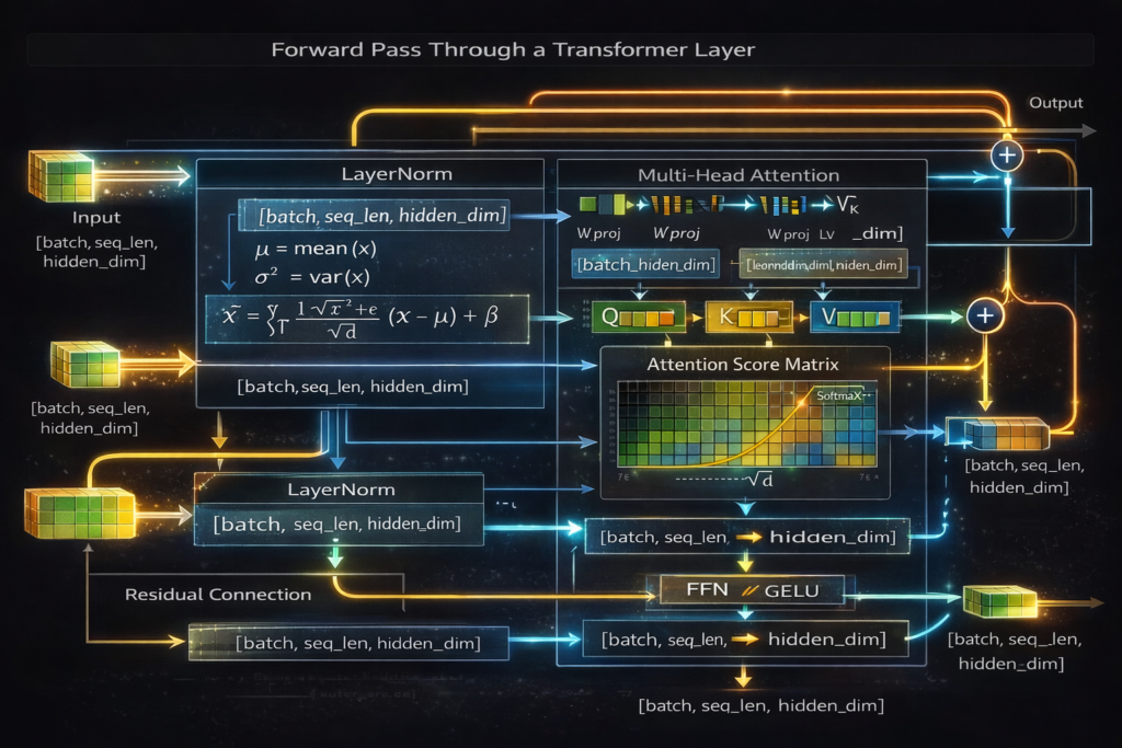
The Forward Pass: From Input to Output

Step 1: Input Embedding Lookup

Given token IDs t1​,t2​,…,tn​ , we retrieve embedding vectors:

E=EmbeddingLookup(t)∈Rn×dmodel​

Where dmodel​ is the hidden dimension (e.g., 12,288 for GPT-3).

Memory Layout: Embedding matrix WE​∈RV×d where V is vocabulary size. This is often the largest single matrix in the model.

Step 2: Positional Encoding

Since transformers process all positions simultaneously (unlike RNNs), we must inject positional information:

RoPE (Rotary Positional Embedding) – Used in modern models (Llama, GPT-4):

f(q,m)=qeimθ

Where m is position, θj​=10000−2j/d , applied via rotation matrices to query/key vectors in attention.

Implementation:

Python

Copy

# Simplified RoPE application
def apply_rope(x, positions, theta_base=10000):
    dim = x.shape[-1]
    freqs = 1.0 / (theta_base ** (torch.arange(0, dim, 2).float() / dim))
    angles = torch.outer(positions, freqs)
    cos, sin = torch.cos(angles), torch.sin(angles)
    
    x1, x2 = x[..., ::2], x[..., 1::2]
    rotated = torch.stack([x1 * cos - x2 * sin, x1 * sin + x2 * cos], dim=-1)
    return rotated.flatten(-2)

Step 3: Transformer Block Processing

Each layer l performs:

Input: h(l)∈Rn×d

Sub-layer 1: Multi-Head Self-Attentiona(l)=LayerNorm(h(l)) h′(l)=h(l)+Attention(a(l),a(l),a(l))

Sub-layer 2: Feed-Forward Networkh′′(l)=LayerNorm(h′(l)) h(l+1)=h′(l)+FFN(h′′(l))

---

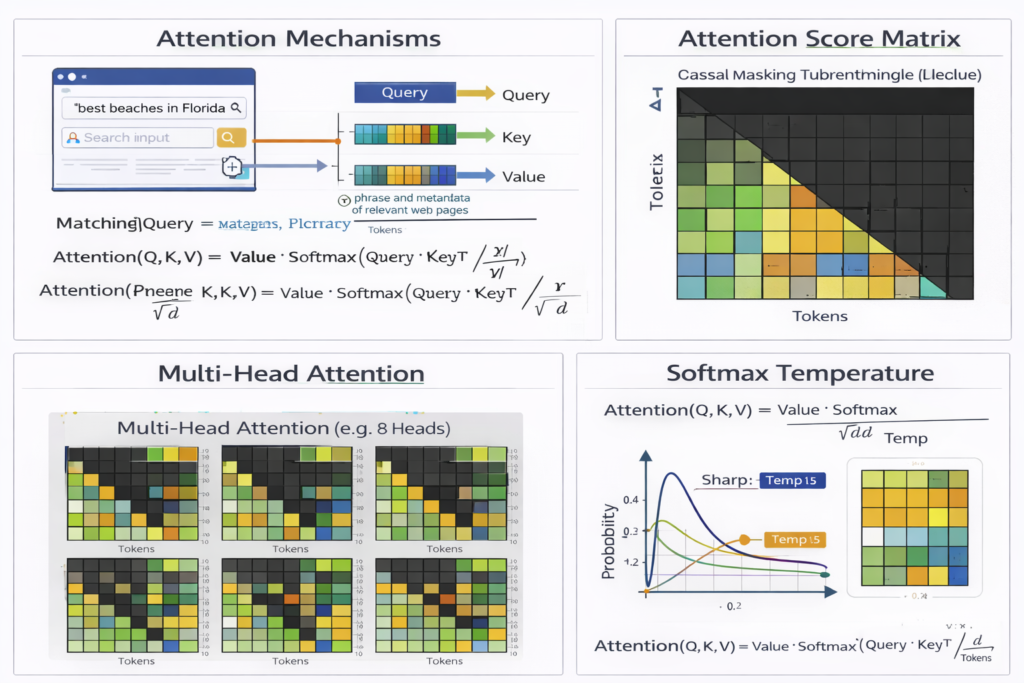
Attention Mechanisms: The Core Innovation

Scaled Dot-Product Attention

The fundamental operation:

Attention(Q,K,V)=softmax(dk​​QKT​)V

Where:

• Q∈Rn×dk​ (Queries)
• K∈Rn×dk​ (Keys)
• V∈Rn×dv​ (Values)
• dk​​ prevents softmax saturation (typically dk​=dmodel​/h )

Multi-Head Attention

Parallel attention computations with different learned projections:

MultiHead(Q,K,V)=Concat(head1​,…,headh​)WO

Where headi​=Attention(QWiQ​,KWiK​,VWiV​)

Computational Complexity: O(n2⋅d) for sequence length n and dimension d . This quadratic scaling is the primary bottleneck for long contexts.

Causal (Autoregressive) Masking

For generation, we apply a triangular mask to prevent attending to future positions:

Mij​={0−∞​if i≥jif i<j​

Attention(Q,K,V)=softmax(dk​​QKT​+M)V

Implementation Optimization: Instead of computing full QKT and masking, modern implementations use Flash Attention—fusing attention computation to reduce memory bandwidth bottlenecks.

---

Layer-by-Layer Processing

Feed-Forward Networks

Each transformer block contains a position-wise FFN:

FFN(x)=GELU(xW1​+b1​)W2​+b2​

SwiGLU Variant (used in Llama, PaLM):

SwiGLU(x)=(SiLU(xW)⊗xV)W2​

Where ⊗ is element-wise multiplication. This uses three matrices instead of two but improves performance.

Dimensions:

• W1​∈Rd×4d (expansion)
• W2​∈R4d×d (projection)

Activation Functions

GELU (Gaussian Error Linear Unit):

GELU(x)=x⋅Φ(x)=x⋅21​[1+erf(2​x​)]

Approximation used in practice: 0.5x(1+tanh[2/π​(x+0.044715x3)])

SiLU/Swish:

SiLU(x)=x⋅σ(x)=1+e−xx​

Layer Normalization

Pre-normalization architecture (used in modern models):

LayerNorm(x)=γ⊙σ2+ϵ​x−μ​+β

Where μ,σ2 are computed across the hidden dimension for each token independently.

---

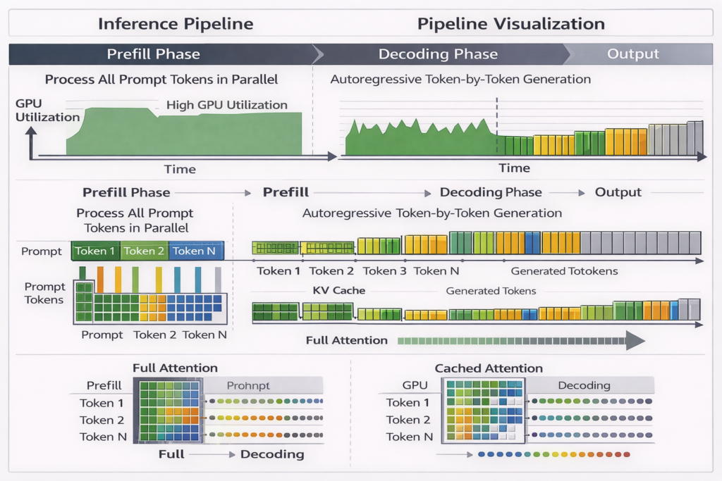
The Inference Pipeline: Step-by-Step

Phase 1: Prefill (Prompt Processing)

Given input prompt of length n :

1. Tokenize: Convert to token IDs →O(n)
2. Embedding Lookup: Fetch embedding vectors →O(n⋅d)
3. Parallel Forward Pass: Process all n tokens simultaneously through all layers
4. Cache Population: Store Key (K ) and Value (V ) tensors for each layer

Computational Characteristics:

• Compute-bound (matrix multiplications)
• GPU utilization: 90%+
• Time complexity: O(n2⋅d⋅L) where L is number of layers

Phase 2: Decoding (Token Generation)

For each new token at position t :

1. Single Token Embedding: O(d)
2. Cached Attention: Reuse K,V from previous tokens
   • Compute new Qt​
   • Attend to cached K1:t​,V1:t​
   • Complexity: O(t⋅d) instead of O(t2⋅d)
3. Feed-Forward: O(d2)
4. Sampling: O(V) (vocabulary size)
5. Cache Update: Store new Kt​,Vt​

KV Cache Memory: For layer l , cache size is 2⋅n⋅dmodel​ (K and V). For 96 layers, 128k context, 12k hidden size: Cache=96×2×131072×12288×2 bytes (fp16)≈590 GB

This necessitates model parallelism and compression techniques (MQA, GQA).

---

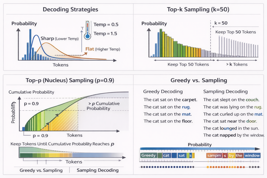
Decoding Strategies: From Probabilities to Text

Logit Computation

Final layer output hfinal​∈Rd projects to vocabulary:

z=hfinal​Wunemb​+bunemb​∈RV

Where Wunemb​∈Rd×V (often tied with input embedding matrix).

Temperature Scaling

Apply temperature T to control randomness:

P(xi​)=∑j​ezj​/Tezi​/T​

• T→0 : Greedy decoding (argmax)
• T=1 : True distribution
• T>1 : More random/creative

Sampling Strategies

Top-k Sampling:

1. Sort logits: z(1)​≥z(2)​≥…≥z(V)​
2. Keep top k , set others to −∞
3. Sample from remaining distribution

Nucleus (Top-p) Sampling:

1. Compute cumulative probability mass
2. Find smallest set V(p) such that ∑i∈V(p)​P(i)≥p
3. Sample from V(p)

Repetition Penalty: z~i​={zi​/αzi​​if token i in contextotherwise​

Where α>1 (typically 1.1-1.2) discourages repetition.

---

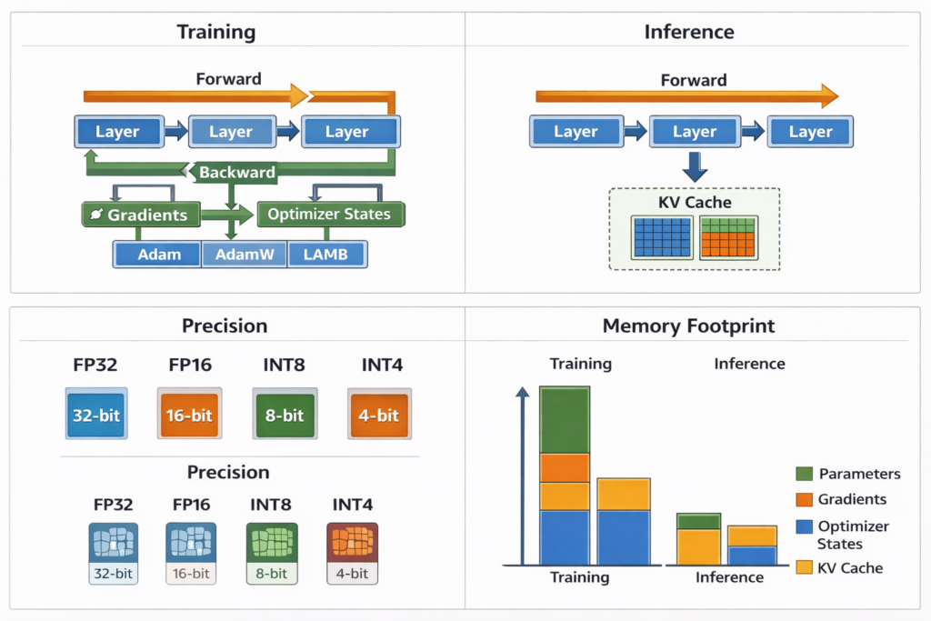
Training vs. Inference: Key Differences

Aspect	Training	Inference
Direction	Forward + Backward	Forward only
Precision	Mixed (BF16/FP32)	Often quantized (INT8/INT4)
Batching	Large batches (millions of tokens)	Variable (1 to batch size)
Attention	Full bidirectional or causal	Causal with KV caching
Memory	Store activations for gradients	Store KV cache
Optimization	Gradient descent	Various decoding strategies
Throughput	Tokens/sec (training)	Time to first token + inter-token latency

Quantization for Inference

GPTQ/AWQ: Post-training quantization to 4-bit weights

minW^​∥WX−W^X∥22​

Where W^ is quantized to 4-bit with grouping (e.g., 128 weights share scale/zero-point).

Activation-aware: Protect sensitive weight channels (outliers) from quantization error.

---

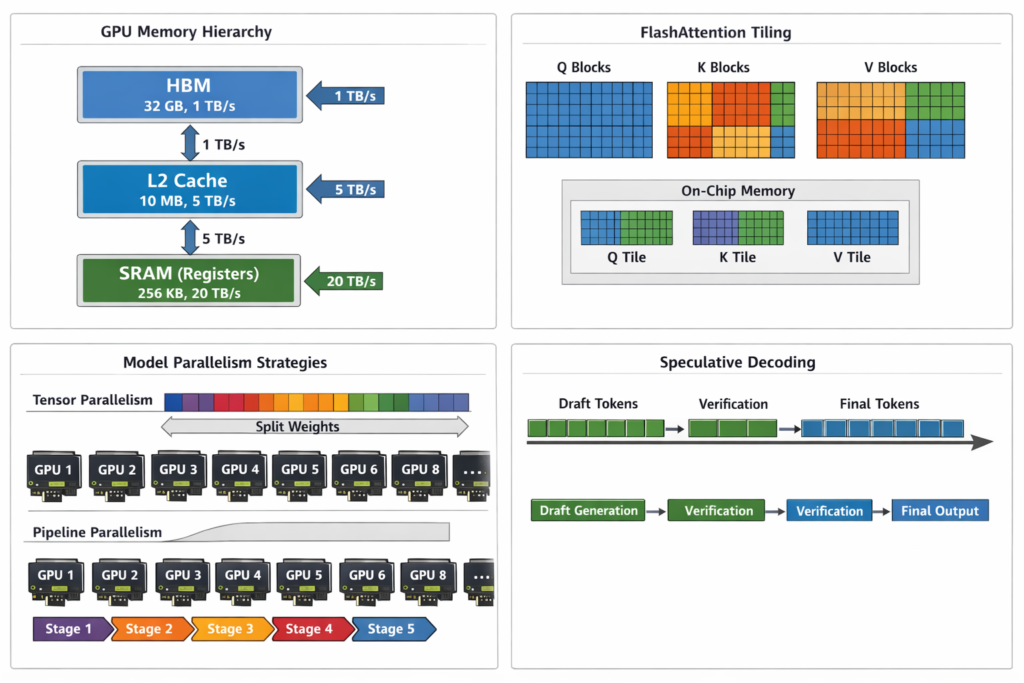
Hardware and Optimization

GPU Kernel Optimization

FlashAttention-2: Algorithmic reformulation of attention to reduce HBM (High Bandwidth Memory) accesses:

• Tiling: Load blocks of Q,K,V into SRAM (faster on-chip memory)
• Online softmax: Compute softmax without materializing full S=QKT matrix
• Recomputation: Recompute attention weights during backward pass instead of storing

Speedup: 2-4× faster than standard attention, 5-20× memory efficient.

Model Parallelism Strategies

Tensor Parallelism: Split individual layers across GPUs

• Column-wise: Split WQ​,WK​,WV​ across devices
• Row-wise: Split WO​ (output projection)

Pipeline Parallelism: Split layers across GPUs

• GPU 0: Layers 0-11
• GPU 1: Layers 12-23
• etc.

Sequence Parallelism: Split sequence dimension for long contexts (Ring Attention).

Speculative Decoding

Use small draft model to predict multiple tokens, verify with large model in parallel:

1. Draft model generates 5 tokens autoregressively (fast)
2. Target model verifies all 5 in one forward pass (parallel)
3. Accept tokens up to first mismatch
4. Resample from adjusted distribution if needed

Speedup: 2-3× for latency-critical applications.

---

Conclusion and Future Directions

The journey from prompt to completion involves a sophisticated orchestration of:

1. Tokenization: Subword segmentation via BPE
2. Embedding: High-dimensional vector representations
3. Positional Encoding: RoPE for relative position awareness
4. Transformer Layers: O(L) sequential applications of attention and FFN
5. Attention Mechanisms: O(n2) operations with KV caching optimization
6. Decoding: Probabilistic sampling with temperature and top-p/nucleus filtering

Each component represents decades of research in neural network architectures, optimization algorithms, and hardware acceleration. The apparent “intelligence” emerges from the statistical regularities captured in hundreds of billions of parameters trained on trillions of tokens—not from symbolic reasoning or consciousness.

Emerging Trends

• Mixture of Experts (MoE): Sparse activation (e.g., GPT-4, Mixtral) reducing inference cost
• Long Context: Ring Attention, linear attention mechanisms for million-token contexts
• Multimodal Integration: Unified architectures processing text, image, audio
• Efficiency: 1-bit quantization, pruning, and hardware-specific optimizations
• Test-Time Compute: Chain-of-thought scaling with additional inference-time computation

Understanding these mechanisms is essential for ML engineers building production systems, optimizing inference latency, or fine-tuning models for specific applications. The transformer architecture, despite its computational intensity, remains the dominant paradigm—though the field continues to evolve toward more efficient and capable architectures.

---

Technical Glossary

• Autoregressive: Generating tokens one at a time, conditioning on previous outputs
• KV Cache: Key-value storage from previous tokens to avoid recomputation
• Logits: Raw, unnormalized model outputs before softmax
• Perplexity: exp(−N1​∑logP(xi​)) , measurement of model confidence
• Temperature: Hyperparameter controlling randomness in sampling
• Zero-shot: Performing tasks without task-specific training examples

---

Technical References:

• Vaswani et al., “Attention Is All You Need” (2017)
• Brown et al., “Language Models are Few-Shot Learners” (2020)
• Su et al., “RoFormer: Enhanced Transformer with Rotary Position Embedding” (2021)
• Dao et al., “FlashAttention: Fast and Memory-Efficient Exact Attention” (2022)

---

This article provides production-level technical accuracy suitable for engineering teams implementing or optimizing LLM inference pipelines. All architectural descriptions reflect current state-of-the-art implementations as of 2024.