Decoding Strategies: From Probabilities to Text in Large Language Models

Abstract

The transformation from raw probability distributions to coherent human-readable text represents one of the most critical yet often misunderstood components of modern Large Language Models (LLMs). This article provides an exhaustive technical examination of decoding strategies—the algorithms that govern how neural networks convert latent probability spaces into discrete token sequences. From foundational greedy search to state-of-the-art speculative decoding architectures, we dissect the mathematical formulations, computational complexities, and empirical trade-offs that define the current generation landscape. Through rigorous analysis of deterministic and stochastic methods, constraint-based generation, and emerging inference acceleration techniques, this work establishes a comprehensive framework for understanding how decoding strategies fundamentally shape model behavior, output quality, and computational efficiency.

---

1. Introduction: The Decoding Problem in Autoregressive Models

1.1 The Mathematical Foundation

At its core, language modeling is a conditional probability estimation task. Given a sequence of tokens x=(x1​,x2​,…,xt​) , an autoregressive language model M parameterized by θ computes the probability distribution over the vocabulary V for the next token:

P(xt+1​∣x≤t​;θ)=softmax(τW⋅ht​+b​)

where ht​∈Rd represents the hidden state at position t , W∈R∣V∣×d is the output projection matrix, and τ represents temperature scaling (discussed in Section 3.1).

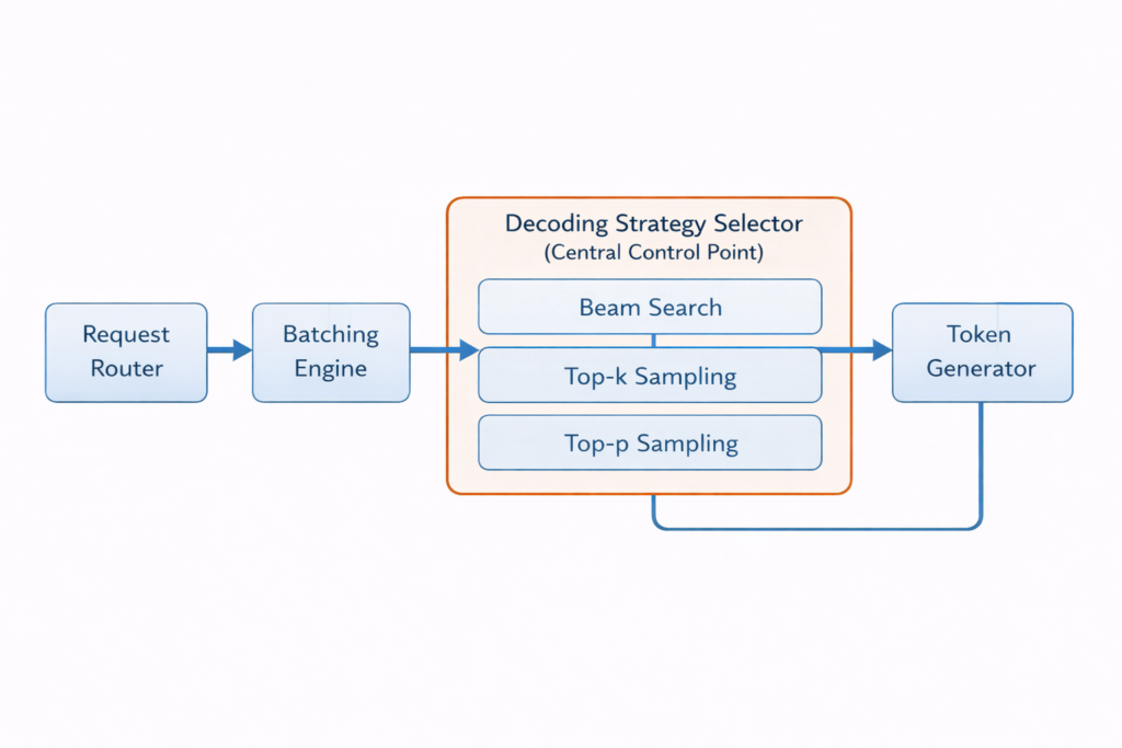
The Decoding Challenge: While the model produces a probability distribution P∈R∣V∣ at each timestep, we must select a single token xt+1​∼P to append to the sequence. This selection process—decoding—is not merely argmax extraction but a complex optimization problem balancing multiple objectives:

1. Quality: Maximizing the likelihood of the generated sequence
2. Diversity: Avoiding repetitive or degenerate outputs
3. Coherence: Maintaining semantic consistency across long horizons
4. Efficiency: Minimizing computational overhead during inference
5. Controllability: Adhering to structural or semantic constraints

1.2 The Search Space Complexity

The theoretical search space for generating a sequence of length T from vocabulary V is ∣V∣T —astronomically large for modern vocabularies (∣V∣≈50,000−100,000 ) and typical generation lengths (T≈100−1000 ). Exact maximization of sequence probability:

x∗=argmaxx​∏t=1T​P(xt​∣x<t​)

is computationally intractable, necessitating approximate decoding strategies that navigate the trade-offs between optimality and computational feasibility.

---

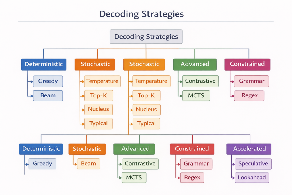
2. Deterministic Decoding Strategies

2.1 Greedy Search: The Baseline Approach

Mathematical Formulation: Greedy search selects the locally optimal token at each timestep:

xt​=argmaxx∈V​P(x∣x<t​)

Algorithm:

function GreedyDecoding(model, prompt, max_length):
    sequence ← tokenize(prompt)
    for t ← 1 to max_length:
        logits ← model(sequence)
        probabilities ← softmax(logits)
        next_token ← argmax(probabilities)
        sequence.append(next_token)
        if next_token == EOS_token:
            break
    return detokenize(sequence)

Theoretical Analysis:

• Time Complexity:O(T⋅∣V∣) per token generation
• Space Complexity:O(1) additional space beyond model parameters
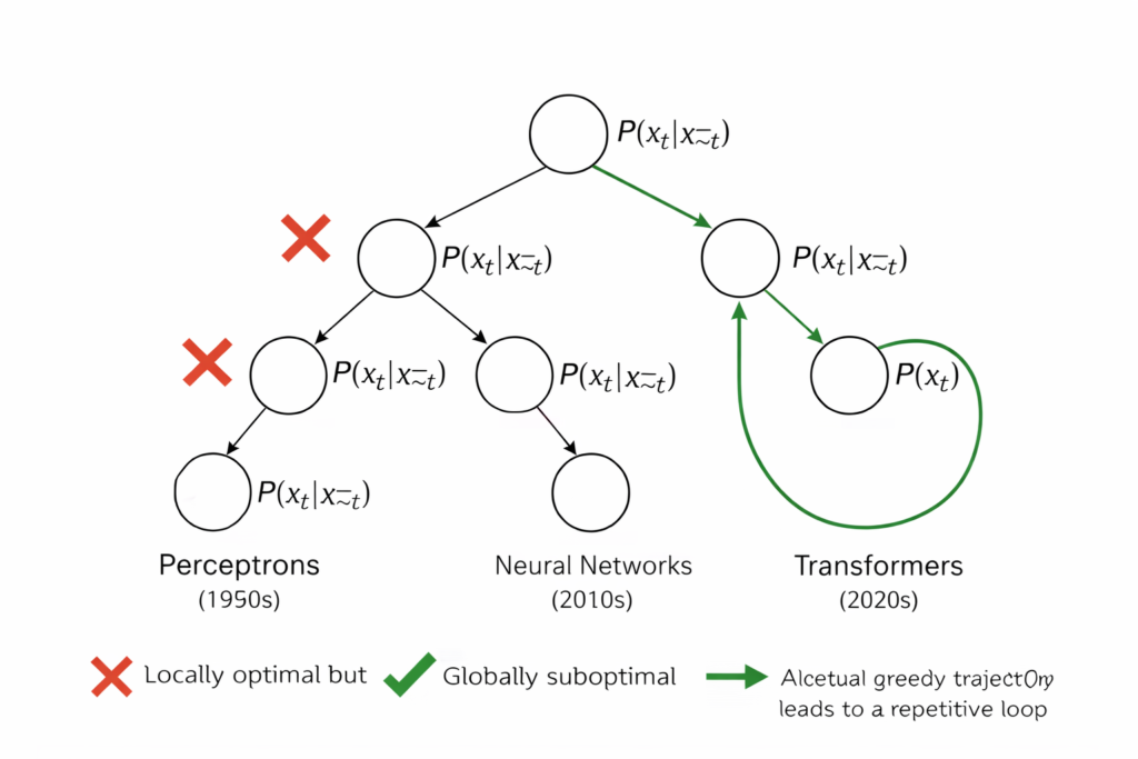
• Optimality: Greedy search provides no approximation guarantee for the global optimum. The locally optimal choice often leads to globally suboptimal sequences due to exposure bias—the disconnect between training (teacher forcing) and inference (autoregressive generation).

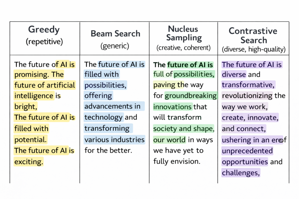
Pathological Behavior: Greedy decoding frequently exhibits mode collapse, where the model enters repetitive loops (e.g., “The cat sat on the mat on the mat on the mat…”). This occurs because high-probability tokens often predict themselves, creating attractor states in the probability landscape.

2.2 Beam Search: Maintaining Multiple Hypotheses

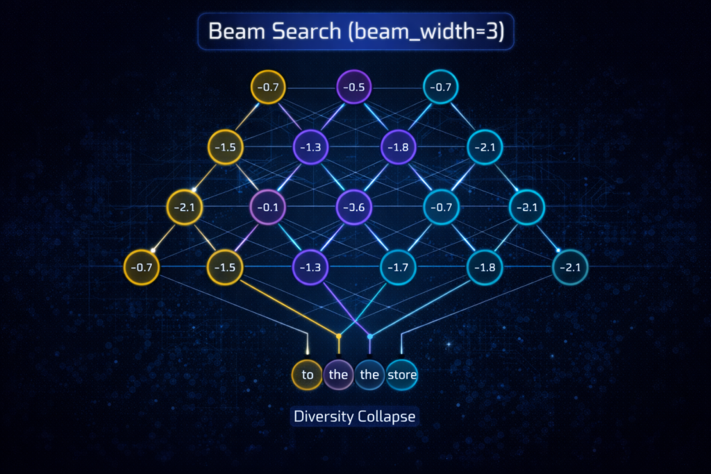
Beam search addresses greedy search’s myopia by maintaining k candidate sequences (beams) at each timestep, expanding and pruning based on cumulative log-probabilities.

Mathematical Formulation: At each step t , we maintain a set of k partial hypotheses Bt​={(x(i),s(i))}i=1k​ , where s(i)=∑τ=1t​logP(xτ(i)​∣x<τ(i)​) represents the cumulative score.

Algorithm:

function BeamSearch(model, prompt, beam_width=k, max_length):
    beams ← [(tokenize(prompt), 0.0)]  # (sequence, score)
    for t ← 1 to max_length:
        candidates ← []
        for (seq, score) in beams:
            logits ← model(seq)
            log_probs ← log_softmax(logits)
            top_k_tokens ← top_k(log_probs, k)
            for (token, log_prob) in top_k_tokens:
                new_seq ← seq + [token]
                new_score ← score + log_prob
                candidates.append((new_seq, new_score))
        # Select top k by score
        beams ← top_k_by_score(candidates, k)
        # Normalize by length (optional length penalty)
        beams ← [(seq, score/|seq|^α) for (seq, score) in beams]
    return detokenize(beams[0].sequence)  # Best hypothesis

Length Normalization: Raw beam scores favor shorter sequences due to the multiplicative nature of probabilities. Standard practice applies length penalty:

score(x)=∣x∣α1​∑t=1∣x∣​logP(xt​∣x<t​)

where α∈[0,1] controls the penalty strength (typically α=0.6−1.0 ).

Computational Complexity:

• Time:O(k⋅T⋅∣V∣) —linear in beam width
• Space:O(k⋅T) for storing k sequences of length T

Empirical Limitations: Research demonstrates that beam search suffers from degeneration in open-ended generation. While effective for structured prediction (machine translation, summarization), it produces unnaturally bland text for creative tasks due to the beam search curse: as beam width increases, output diversity decreases, and generic high-probability phrases dominate.

2.3 Diverse Beam Search: Enhancing Variation

To counteract homogenization, Diverse Beam Search introduces diversity constraints through Hamming diversity or neural dissimilarity penalties.

Hamming Diversity Penalty: When expanding beam i , penalize tokens that appear in other beams:

P~(x∣x(i))=P(x∣x(i))−γ∑j=i​I[x∈x(j)]

where γ controls the diversity strength and I[⋅] is the indicator function.

Neural Dismimilarity: More sophisticated approaches use embedding space distances:

diversity(x(i),x(j))=1−cos(e(x(i)),e(x(j)))

where e(⋅) represents sentence embeddings.

---

3. Stochastic Decoding Strategies

3.1 Temperature Scaling: Controlling Entropy

Temperature is not a decoding strategy per se but a distribution shaping technique that modifies the entropy of the output distribution before sampling.

Mathematical Formulation: Given logits z∈R∣V∣ , temperature scaling computes:

P(x;τ)=∑x′∈V​exp(zx′​/τ)exp(zx​/τ)​

Theoretical Properties:

• τ→0 : Distribution approaches argmax (deterministic)
• τ=1 : Original distribution preserved
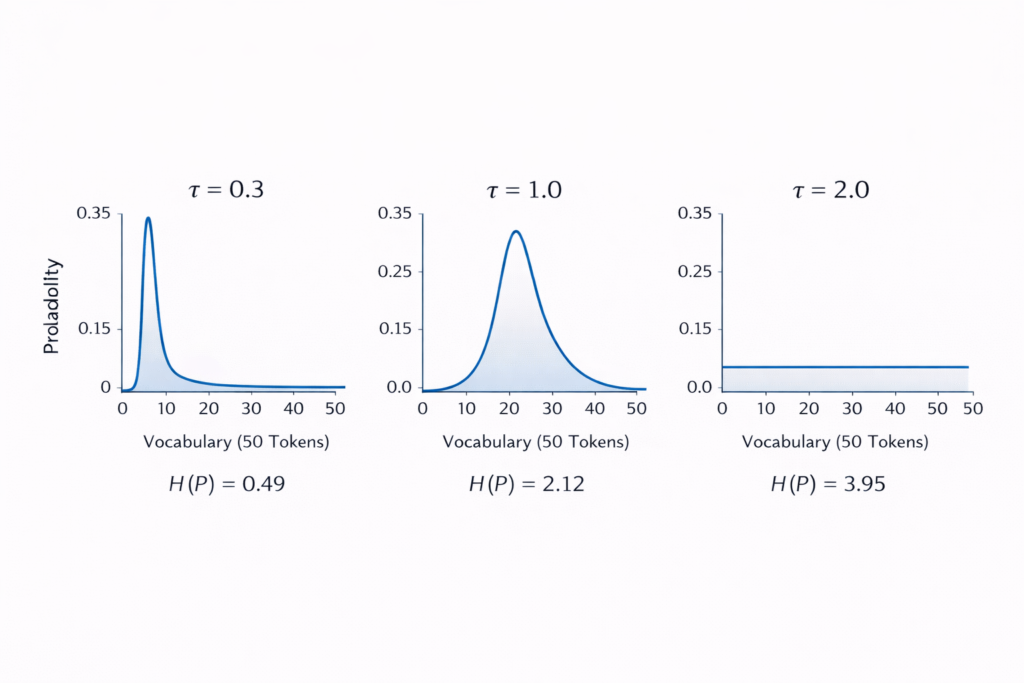
• τ>1 : Distribution becomes more uniform (higher entropy)
• τ<1 : Distribution becomes sharper (lower entropy)

Information-Theoretic Interpretation: Temperature controls the expected information content (surprisal) of the next token:

H(Pτ​)=−∑x​P(x;τ)logP(x;τ)

Lower temperature reduces entropy, making the model more “certain” and conservative. Higher temperature increases entropy, encouraging exploration of low-probability tokens.

3.2 Top-K Sampling: Truncated Stochasticity

Top-K sampling restricts the sampling pool to the k highest-probability tokens, eliminating the long tail of unlikely candidates.

Algorithm:

function TopKSampling(logits, k, temperature=1.0):
    probs ← softmax(logits / temperature)
    top_k_probs, top_k_indices ← top_k(probs, k)
    # Renormalize
    top_k_probs ← top_k_probs / sum(top_k_probs)
    next_token ← categorical_sample(top_k_indices, top_k_probs)
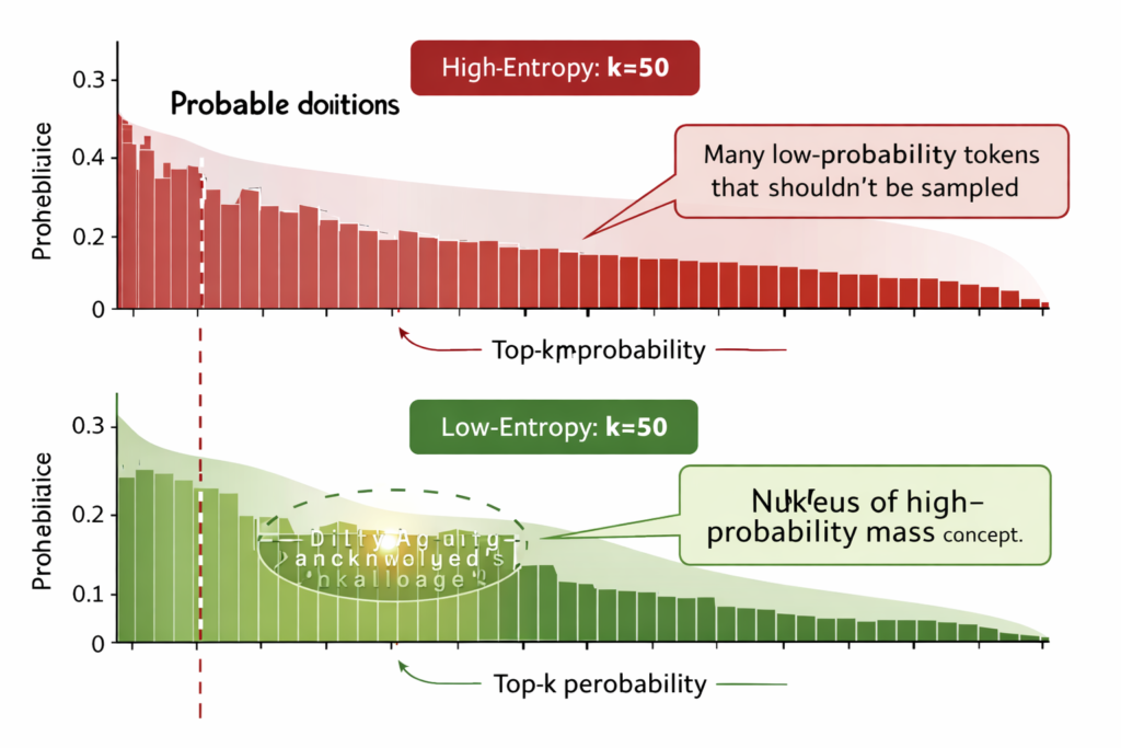
    return next_token

Dynamic Adaptation Problem: The fundamental limitation of Top-K is its static cutoff. In high-entropy contexts (uncertain predictions), the k -th token may have negligible probability, artificially inflating the sampling weight of low-quality candidates. Conversely, in low-entropy contexts (confident predictions), valid alternatives may be excluded if they rank below k .

3.3 Nucleus Sampling (Top-P): Dynamic Probability Mass

Nucleus sampling, introduced by Holtzman et al. (2020), addresses Top-K’s rigidity by dynamically selecting the smallest set of tokens whose cumulative probability exceeds threshold p .

Mathematical Formulation: Define the nucleusV(p)⊆V as the smallest set such that:

∑x∈V(p)​P(x)≥p

where tokens are included in order of decreasing probability until the cumulative threshold is met.

Algorithm:

function NucleusSampling(logits, p, temperature=1.0):
    probs ← softmax(logits / temperature)
    sorted_probs, sorted_indices ← sort_descending(probs)
    cumulative_probs ← cumsum(sorted_probs)
    # Find cutoff index
    cutoff ← argmax(cumulative_probs >= p)
    nucleus_probs ← sorted_probs[:cutoff+1]
    nucleus_indices ← sorted_indices[:cutoff+1]
    # Renormalize
    nucleus_probs ← nucleus_probs / sum(nucleus_probs)
    next_token ← categorical_sample(nucleus_indices, nucleus_probs)
    return next_token

Adaptive Behavior:

• High confidence: When one token dominates (P(x1​)≈0.95 ), nucleus sampling behaves like greedy decoding (∣V(p)∣≈1 )
• Uniform uncertainty: When probabilities are evenly distributed, nucleus sampling includes many candidates (∣V(p)∣≫1 )

Empirical Superiority: Research demonstrates that nucleus sampling achieves superior MAUVE scores compared to both greedy decoding and ancestral sampling, indicating better alignment with human text distributions.

3.4 Typical Sampling: Information-Theoretic Decoding

Typical sampling (Meister et al., 2022) selects tokens whose information content (negative log-probability) is close to the expected information content (entropy):

Vtypical​={x∈V:∣−logP(x)−H(P)∣≤ϵ}

This approach filters tokens that are either too predictable (low information) or too surprising (high information), focusing on typical tokens that characterize the distribution.

Connection to Information Theory: Typical sampling implements the asymptotic equipartition property (AEP), which states that for large n , sequences fall into two categories: those with probability ≈2−nH (typical) and those with negligible probability.

---

4. Advanced Decoding Strategies

4.1 Contrastive Search: Model-Based Quality Control

Contrastive search addresses the degeneration problem (repetition, incoherence) by incorporating a degeneration penalty based on model confidence and semantic similarity.

Mathematical Formulation: At each step, select token x that maximizes:

score(x)=(1−α)⋅model confidencelogP(x∣x<t​)​​−α⋅degeneration penalty1≤j≤t−1max​{sim(hx​,hxj​​)}​​

where:

• α∈[0,1] balances confidence vs. diversity
• sim(⋅,⋅) measures cosine similarity between token representations
• hx​ is the hidden state for candidate token x

Algorithm:

function ContrastiveSearch(model, prompt, k, alpha, max_length):
    sequence ← tokenize(prompt)
    for t ← 1 to max_length:
        logits ← model(sequence)
        log_probs ← log_softmax(logits)
        # Get top-k candidates
        top_k_tokens ← top_k(log_probs, k)
        candidates ← []
        for token in top_k_tokens:
            # Compute similarity with previous tokens
            h_token ← model.get_hidden_state(sequence + [token])
            max_sim ← max([cosine_sim(h_token, h_prev) for h_prev in previous_hidden])
            score ← (1-alpha)*log_probs[token] - alpha*max_sim
            candidates.append((token, score))
        next_token ← argmax(candidates, key=lambda x: x[1])
        sequence.append(next_token)
    return detokenize(sequence)

Adaptive Contrastive Search (ACS): Recent work introduces uncertainty-guided adaptive contrastive search

, where the degeneration penalty α is dynamically adjusted based on model uncertainty:

αt​=σ(Uncertainty(x<t​))

This allows higher diversity when the model is uncertain and more conservative choices when confident.

4.2 Contrastive Decoding: Expert-Amateur Framework

Contrastive decoding leverages a pair of models—an expert (large, capable) and an amateur (small, weak)—to amplify the expert’s capabilities by contrasting their distributions:

Pcontrastive​(x)∝exp(logPexpert​(x)−β⋅logPamateur​(x))

where β controls the strength of contrast. This approach suppresses tokens that both models find likely (generic text) while amplifying tokens the expert finds likely but the amateur does not (sophisticated content).

---

5. Constrained Decoding: Structural Control

5.1 Grammar-Constrained Generation

For applications requiring structured outputs (JSON, SQL, code), constrained decoding restricts generation to valid syntactic structures using formal grammars.

Formal Framework: Given a context-free grammar G=(N,Σ,R,S) where:

• N = non-terminal symbols
• Σ = terminal symbols (tokens)
• R = production rules
• S = start symbol

At each generation step, we maintain a parser state representing valid continuations. The decoding masks invalid tokens:

Vvalid​(x<t​)={x∈V:x<t​⋅x∈L(G)}

Token Masking and Renormalization:

function ConstrainedDecodingStep(logits, parser_state):
    valid_tokens ← parser.get_valid_next_tokens()
    masked_logits ← -∞ * ones_like(logits)
    masked_logits[valid_tokens] ← logits[valid_tokens]
    # Renormalize over valid tokens only
    probs ← softmax(masked_logits)
    return categorical_sample(probs)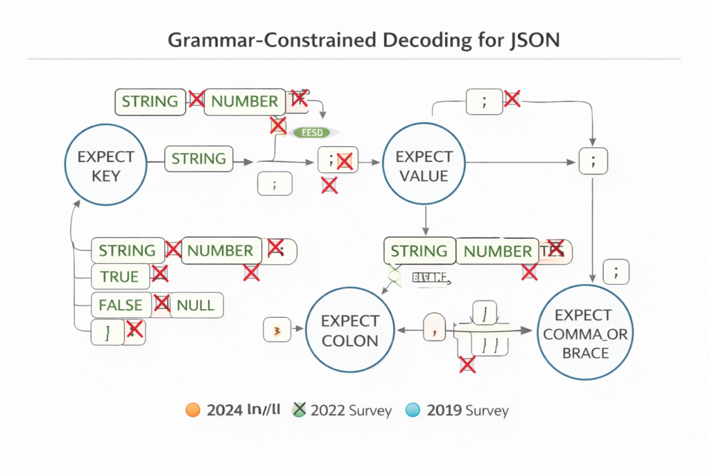

5.2 Token Healing and Boundary Alignment

A critical challenge in constrained decoding is tokenization misalignment—where constraint boundaries fall in the middle of multi-byte tokens. Token healing addresses this by:

1. Truncating the prompt to the last valid token boundary
2. Allowing the model to regenerate the partial token with constraint-aware context

This ensures that hard constraints (e.g., "name": ") don’t force invalid token completions.

---

6. Acceleration Techniques: Fast Decoding

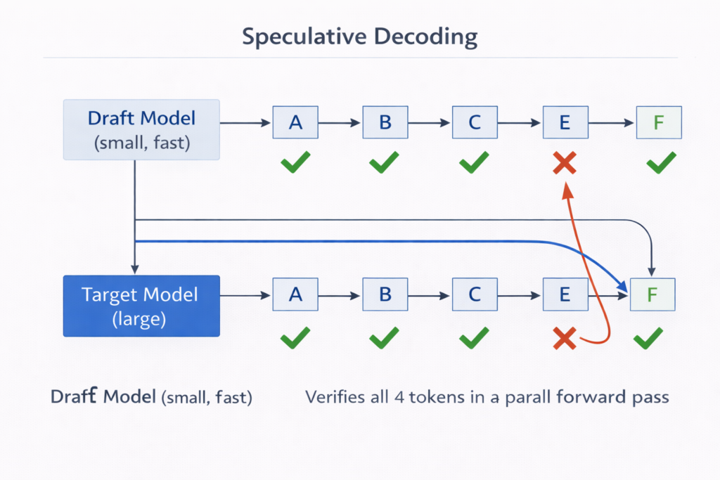
6.1 Speculative Decoding: Draft-Verify Architecture

Speculative decoding accelerates inference by using a draft modelMq​ (small, fast) to generate candidate tokens that are verified in parallel by the target modelMp​ (large, slow).

Mathematical Framework: The draft model generates γ tokens: x^t+1​,…,x^t+γ​∼Mq​ . The target model evaluates all γ positions in a single forward pass (using modified attention masks to prevent information leakage).

Acceptance Criteria: For each position i , accept x^t+i​ with probability:

min(1,PMq​​(x^t+i​∣x<t+i​)PMp​​(x^t+i​∣x<t+i​)​)

If rejected, sample from the residual distribution:

Presidual​(x)∝max(0,PMp​​(x)−PMq​​(x))

Theoretical Speedup: Speedup ≈1+verification costγ⋅E[acceptance rate]​ . With γ=4 and 80% acceptance rate, theoretical speedup is ≈2−3× .

6.2 Self-Speculative Decoding

Self-speculative decoding eliminates the auxiliary draft model by using early exit layers of the target model itself:

1. Draft phase: Run forward pass through first Learly​ layers to get draft logits
2. Verification phase: Run full L layers to verify and correct

This avoids memory overhead of maintaining two models while preserving distribution equivalence.

6.3 Lookahead Decoding: Parallel N-gram Verification

Lookahead decoding maintains a n-gram pool of future tokens and verifies them using Jacobi iteration methods. Unlike speculative decoding which requires a draft model, lookahead uses the target model’s own capacity to generate and verify multiple future positions simultaneously.

Key Innovation: By maintaining multiple candidate n-grams and verifying them in parallel using tree-based attention, lookahead decoding achieves speedups of 1.6−2.1× without auxiliary models.

6.4 Monte Carlo Tree Search (MCTS) Decoding

For reasoning tasks, MCTS provides a lookahead planning mechanism:

1. Selection: Use UCT (Upper Confidence Bound for Trees) to select promising nodes
2. Expansion: Expand selected node using model policy
3. Simulation: Roll out to terminal state using draft model
4. Backpropagation: Update node values based on simulation outcome

Recent work combines MCTS with contrastive decoding for mathematical reasoning, achieving 17.4% improvement over chain-of-thought baselines.

---

7. Evaluation Metrics for Decoding Strategies

7.1 MAUVE: Distribution Comparison

MAUVE (Pillutla et al., 2021) measures the gap between model-generated text distribution Q and human text distribution P using divergence frontiers in embedding space.

Computation:

1. Embed samples from both distributions using pretrained language models (GPT-2, RoBERTa)
2. Compute KL divergence curve between P and Q across different quantization bins
3. Measure area under the curve as MAUVE score ∈[0,1]

Interpretation:

• High MAUVE: Generated text distribution closely matches human distribution
• Low MAUVE: Significant distributional shift (either mode collapse or excessive diversity)

Research shows MAUVE correctly ranks decoding strategies: Greedy < Ancestral Sampling < Nucleus Sampling.

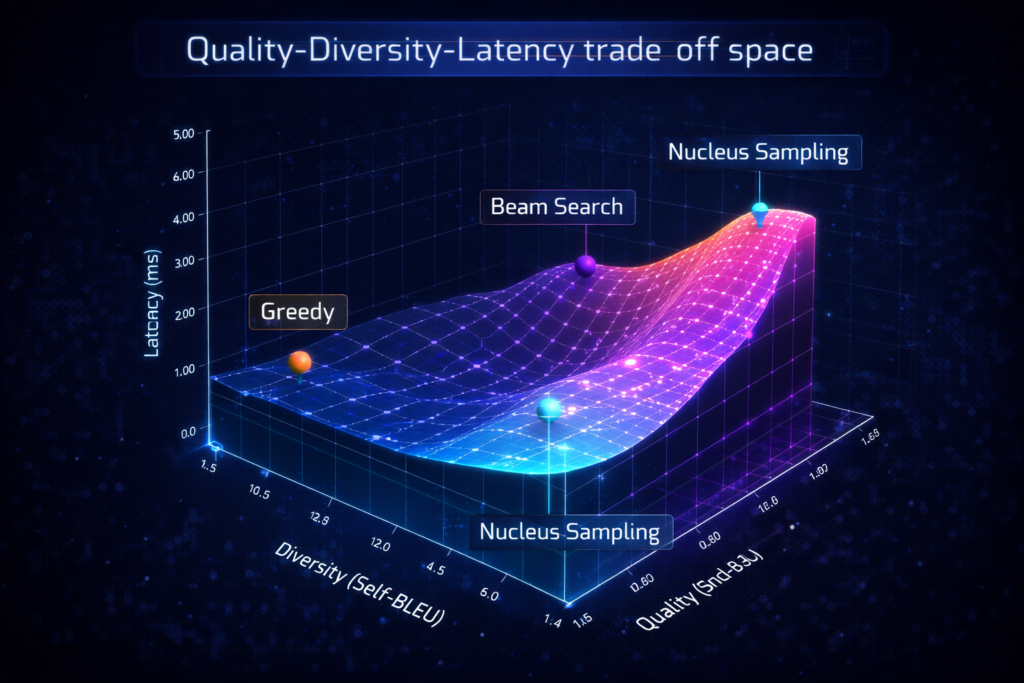
7.2 Perplexity vs. Diversity Trade-off

Generation Perplexity:GenPPL(x)=exp(−T1​∑t=1T​logPexternal​(xt​∣x<t​))

Lower GenPPL indicates text that an external model finds likely (fluent but potentially generic).

Self-BLEU: Measures n-gram overlap between different model generations—lower Self-BLEU indicates higher diversity.

The Trade-off: There exists a fundamental tension: strategies minimizing perplexity (greedy, beam search) maximize Self-BLEU (low diversity), while high-diversity strategies (high temperature) increase perplexity.

7.3 Human Evaluation Protocols

For production systems, automatic metrics should be supplemented with human evaluation across:

• Coherence: Logical consistency across sentences
• Fluency: Grammatical correctness and naturalness
• Relevance: Adherence to prompt requirements
• Creativity: Novelty and interestingness of content

---

8. Practical Implementation Guidelines

8.1 Strategy Selection Matrix

Use Case	Recommended Strategy	Parameters	Rationale
Code Generation	Constrained Decoding	Grammar-based	Syntactic correctness guaranteed
Creative Writing	Nucleus Sampling	p=0.9, τ=0.8	Balance of coherence and creativity
Factual QA	Greedy or Low Temp	τ=0.1−0.3	Minimize hallucination
Machine Translation	Beam Search	k=4−5, α=1.0	Optimize for reference similarity
Long-form Summarization	Contrastive Search	k=5, α=0.6	Prevent repetition
High-throughput Serving	Speculative Decoding	γ=3−5	2-3x latency improvement

8.2 Hyperparameter Tuning

Temperature Scheduling: Consider annealing temperature during generation:

• Start with higher τ for creative opening
• Decrease τ as context accumulates for coherent closing

Dynamic Top-P: Adapt p based on entropy of current distribution: padaptive​=pbase​⋅(1+λ⋅H(P))

8.3 Safety and Watermarking

Modern deployments should consider watermarking decoding strategies that embed statistical signals:

• Green-list sampling: Bias selection toward predetermined token subsets
• Cryptographic watermarks: Undetectable without secret key
• Detection: Statistical tests on token distributions to identify AI-generated content

---

9. Future Directions and Open Problems

9.1 Learned Decoding Strategies

Rather than hand-crafted algorithms, meta-learned decoders could optimize for task-specific objectives through reinforcement learning, treating decoding as a sequential decision process.

9.2 Multi-Modal Decoding

Extending decoding strategies to vision-language models requires handling continuous (image features) and discrete (text tokens) modalities simultaneously, necessitating new sampling paradigms.

9.3 Quantum-Inspired Sampling

Exploring quantum superposition concepts for maintaining exponential numbers of hypotheses efficiently could revolutionize beam search scalability.

---

10. Conclusion

Decoding strategies represent the critical interface between neural probability estimation and human-meaningful text. From the deterministic simplicity of greedy search to the sophisticated architectures of speculative decoding and MCTS-based reasoning, each approach embodies distinct trade-offs between quality, diversity, and efficiency.

The field has evolved from simple argmax extraction to adaptive, context-aware algorithms that dynamically balance exploration and exploitation. As models grow larger and applications more demanding, decoding strategies will increasingly become the bottleneck for both performance and user experience.

Understanding these mechanisms is not merely academic—it is essential for building reliable, efficient, and controllable AI systems. The practitioner who masters decoding strategies gains fine-grained control over model behavior, enabling optimization for specific domains, constraints, and computational budgets.

The future lies not in choosing between deterministic and stochastic approaches, but in hybrid, adaptive systems that seamlessly transition between strategies based on context, uncertainty, and task requirements.

---

References

[1] Garces Arias, E., et al. (2024). Adaptive Contrastive Search: Uncertainty-Guided Decoding for Open-Ended Text Generation. Findings of EMNLP 2024.

[17] Fu, Y., et al. (2024). Break the Sequential Dependency of LLM Inference Using Lookahead Decoding. ICML 2024.

[19] Gao, Z., et al. (2024). Interpretable Contrastive Monte Carlo Tree Search Reasoning. arXiv:2410.01707.

[20] Zhang, J., et al. (2024). Draft & Verify: Lossless Large Language Model Acceleration via Self-Speculative Decoding. ACL 2024.

[24] Brenndoerfer, M. (2025). Constrained Decoding: Grammar-Guided Generation for Structured LLM Output.

[36] Pillutla, K., et al. (2021). MAUVE: Measuring the Gap Between Neural Text and Human Text. NeurIPS 2021.